The Architecture of the Machine Learning Lifecycle

In the pursuit of building intelligent systems, it is a common misconception to view Machine Learning (ML) purely as the act of training algorithms. In reality, model training is but a single cog in a much larger, continuous engineering machine. To ensure models are scalable, reliable, and practically useful, we must adhere to a structured sequence of operations known as the Machine Learning Lifecycle.

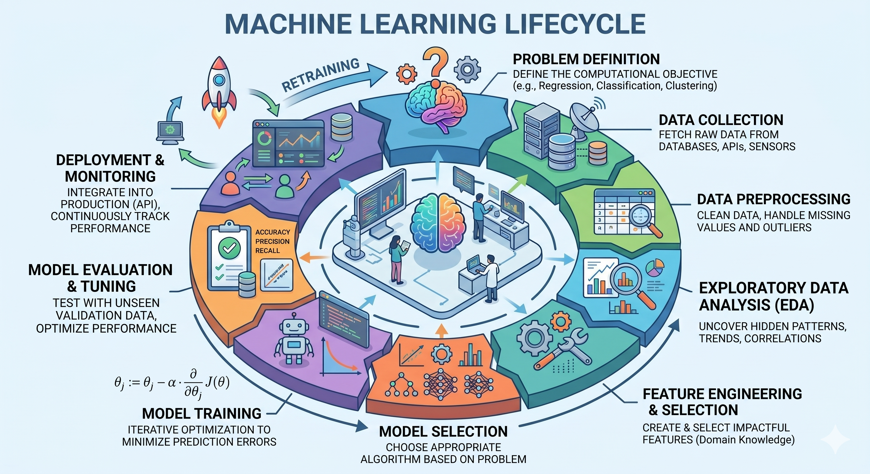
Documenting my journey into the systemtic aspects of ML, this post explores the end-to-end pipeline required to transition a theoretical predictive model from an initial business problem into a robust production environment.

1. Problem Definition and Data Collection

Before writing a single line of code, the overaching objective must be formalized. This involves collaborating with stakeholders to translate a nebulous business requirement (e.g., “reduce customer churn”) into a mathematically optimizable machine learning problem (e.g., “binary classification of user retention probability”). Success criteria and project scope are established here.

• Define the Objective: Every project must begin by translating a real-world goal into a computationally solvable problem. Is the system predicting a continuous value (Regression), categorizing items (Classification), or finding hidden structures (Clustering)?
• Indentify Data Sources: Determine where the necessary information resides. This could be structured relational databases, real-time API streams, or unstructured flat files.
• Collect the Data: Fetch the raw datasets. From a low-level systems perspective, collecting data requires careful consideration of I/O operations and memory limits, especially when streaming large multidimensional arrays into RAM.

2. Data Preprocessing and Feature Engineering

Raw data is inherently noisy and unstructured. Feeding it directly into a mathematical model will cause the system to fail to process it meaningfully.

• Data Cleaning: This step addresses missing values, remove duplicates, and handles extreme outliers that could skew mathematical calculations.
• Data Transformation: Standardize and scale numerical values so that large variables do not dominate smaller ones in distance-based algorithms. Categorical text data is also encoded into binary matrices.
• Exploratory Data Analysis (EDA): Use statistical techniques to uncover underlying patterns, correlations, and trends hidden with the raw information.
• Feature Engineering: This is the most critical engineering phase. It involves translating domain knowledge into a refined numerical matrix, creating new variables that better represent the underlying problem, and selecting only the most impactful features to optimize computational complexity.

3. Model Selection and Iterative Training

With a clean, engineered data matrix ready, the lifecycle transitions into the core algorithmic phase.

• Model Selection: Choose an appropriate baseline algorithm based on the defined problem. A simple linear hypothesis might suffice for basic trends, while a deep neural network is required for complex, unstructured data like images.
• Model Training: This is an iterative optimization process. The algorithm analyzes the training data and adjusts its internal parameters (weights) to minimize prediction errors.
• Mathematical Optimization: Consider the Gradient Descent algorithm, which relies on calculus. Using the partial derivative of a loss function $J(\theta)$, the model finds the steepest path to the minimum error. The parameter update rule is defined as:

\[\theta_{j} := \theta_{j} - \alpha \cdot \frac{\partial}{\partial \theta_{j}} J(\theta)\]

Where the learning rate $\alpha$ dictates the step size. This loop continues until the model’s error converges to a minimum.

4. Evaluation, Deployment, and Continuous Monitoring

A mathematically sound model is useless if it fails in production. The final stages bridge the gap between theory and real-world application.

• Model Evaluation: Before deployment, the model is rigorously tested against a completely unseen dataset (testing set). Metrics like accuracy, precision, and recall are calculated to ensure it generalizes well and hasn’t just memorized the training data.
• Model Deployment: The validated model is integrated into a live production environment. It is often wrapped insided a scalable API pipeline, ready to receive incoming real-time requests and return predictions.
• Monitoring and Maintainance: The lifecycle is cyclical. Once deployed, live data can change over time (known as data drift or concept drift), causing the model’s performance to degrade.
• Retraining: When monitoring systems detect a significant drop in accuracy, the model must be updated with fresh data and retrained, bringing the workflow right back to the begining of the lifecycle.