Data Compression Algorithms

Imagine you need to send a 50 MB file to a friend, but your connection is painfully slow. Or picture a server storing millions of images - without compression, costs would be astronomical. Every time you download a ZIP file, stream a YouTube video, or send a photo on Messenger, data compression algorithms are silently working behind the scenes to make it all possible. In this post, I’ll walk through the core concepts - from the elegantly simple RLE to the surprisingly clever Adaptive Huffman - with real low-level implementations and diagrams to make everything click.

1. What is Data Compression?

At its core, data compression is the process of encoding information using fewer bits than the original representation. Think of it like packing a suitcase: a skilled traveler rolls their clothes instead of folding them flat, fitting twice as much into the same bag.

Two Fundamental Categories

Every compression algorithms falls into one of two camps:

• Lossless compression: the data is perfectly reconstructable after decompression. Not a single bit of information is lost. This works best for text and data files where precision matters. Some notable algorithms include: RLE, LZW, Huffman, ZIP, PNG.
• Lossy compression: some information is permanently discarded to achieve higher compression ratios. The tradeoff is acceptale quality loss. These algorithms are usually applied to multimedia files, where some loss of detail can be tolerated. Some techniques include: JPEG (images), MP3 (audio), MPEG(video).

For this post, we’ll focus entirely on lossless algorithms, which are the workhorses of software, text, and archival compression.

Measuring Compression Efficiency

Before we dive in, let’s define out ruler. The compression ratio $D$ is defined as:

\[D = \frac{N - M}{N} \times 100\%\]

where $N$ is the original data size and $M$ is the compressed size. A higher $D$ means better compression. A $D$ of 50% means you cut the file size in half. The efficiency depends on both the algorithm chosen and the characteristics of the input data.

2. Run-Length Encoding (RLE) - The Simplest One

The Core Idea

RLE is the “Hello World” of compression algorithms. Its principle is disarmingly simple: if a character repeats consecutively, instead of storing every single copy, store the count followed by the character.

Each consecutive sequence of repeated characters is called a run, and it is encoded as:

[count][character]

The longer the run, the higher the compression ratio.

A Quick Example

Input:  AAABBCCAAADE
Output: 3A2B2C3A1D1E

The original string has 12 characters. The encoded version has 12 characters too in this case (counting digits), but imagine a bitmap image with large blocks of the same color - RLE shines brilliantly there.

Assessment

Criterion	Verdict
Simplicity	✅ Extremely simple to implement
Best case	✅ Data with long repeated runs (monochrome images, fax data)
Worst case	❌ Random data — output can be larger than input!
Use cases	BMP images, simple graphics, PCX format

RLE is a fantastic starting point, but it only exploits local repetition. To handle more complex patterns, we need smarter approaches.

3. Lempel-Ziv-Welch (LZW) - The Dictionary Builder

LZW was originally proposed by Ziv and Lempel in 1978 as the LZ78 algorithm, then significantly improved by Terry Welch. It’s a dictionary-based compression algorithm - instead of counting runs, it builds a vocabulary of recurring substrings on the fly. We might already be using LZW every day without knowing it: the GIF and TIFF image formats both rely on it.

The Core Idea

Think of LZW as a shorthand system that two people agree to build together as they talk. Every time a new phrase is coined, it gets added to a shared dictionary and can be referenced by a short code number from that point on.

The encoder maintains a dictionary (initially seeded with all single characters) and greddily matches the longest known substring, emitting its code, then adding a new entry for the next longer string.

The Compression Algorithm (Pseudocode)

w ← NULL
while (READ character k):
  if (wk EXISTS in DICTIONARY):
    w = wk
  else:
    OUTPUT code(w)
    ADD wk to DICTIONARY
    w ← k
OUTPUT code(w)

Worked Example

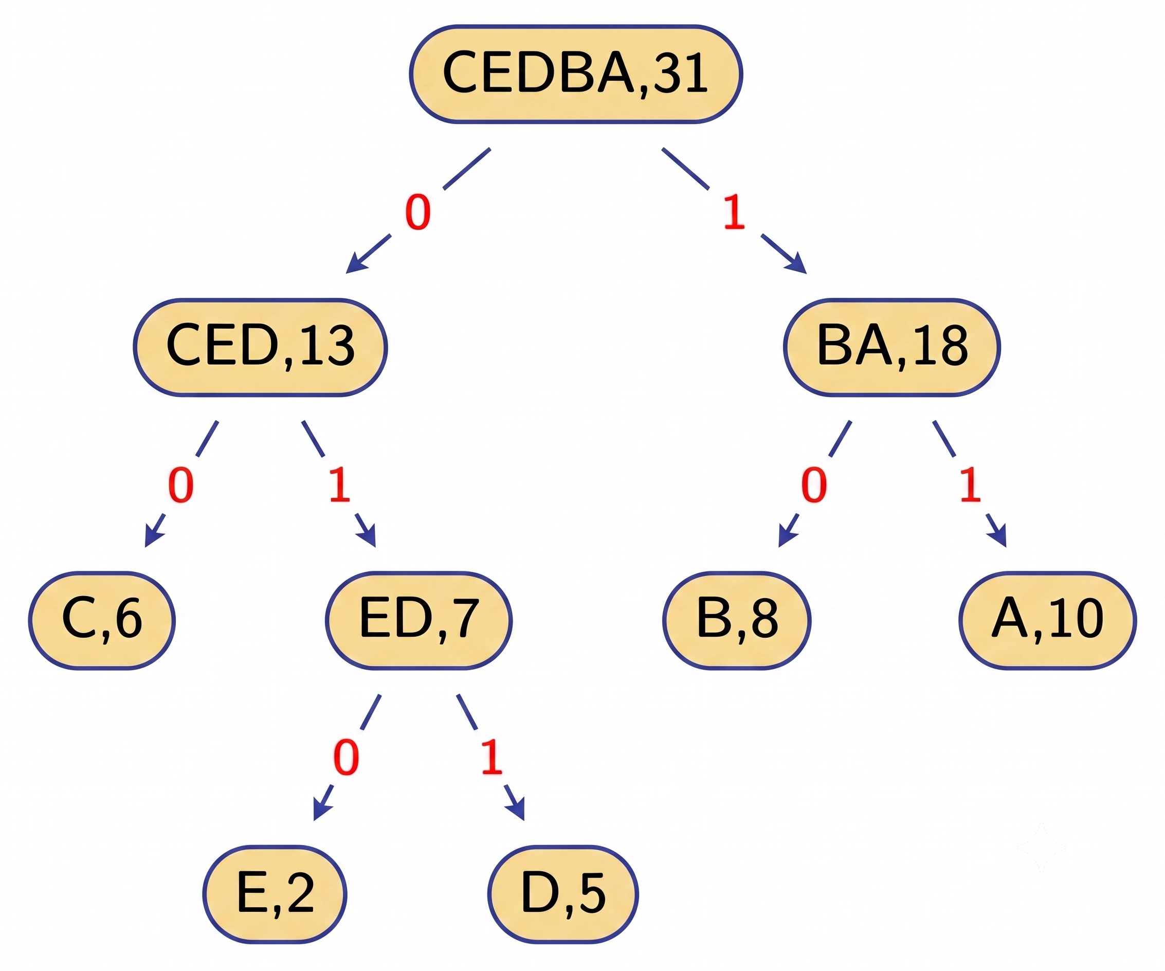
Let’s trace through the encoding of "abracadabarabra" step by step. The dictionary is pre-seeded with codes 0 - 4 for a, b, c, d, r respectively.

The final output code sequence is: 0 1 4 0 2 0 3 5 0 7 6 0

Notice how in the later passes, multi-character patterns like ab (code 5) and ra (code 7) are reused - that’s LZW compression at work.

The Dictionary Tree

Internally, the LZW dictionary if often implemented as a trie (prefix tree), where each path form root to node represents a recognized substring.

Decompression Algorithm

The elegance of LZW is that the decompressor reconstructs the dictionary itself - it doesn’t need the dictionary to be sent alongside the compressed data. The decompressor mirrors the encoder’s logic, rebuilding the same dictionary from the output codes alone.

READ code c
w ← WORD(c)
OUTPUT w
while (READ code c):
  if (c EXISTS in DICTIONARY):
    tmp ← w
    w ← WORD(c)
    ADD (tmp + w[0]) to DICTIONARY
  else:
    ADD (w + w[0]) to DICTIONARY
    w ← WORD(c)
  OUTPUT w

Assessment

• ✅ Dictionary builds automatically — no pre-scanning required
• ✅ Used in GIF, TIFF, compress (Unix)
• ✅ Effective on text and data with repeating patterns
• ⚠️ Dictionary growth can become memory-intensive
• ❌ Patented (expired) — led to creation of PNG as a free alternative

4. Huffman Coding - The Optimal Code

The Big Idea

David Huffman published his algorithm in 1952 while a graduate student at MIT, and it remains one of the most elegant results in information theory. The insight is simple but profound:

Assign shorter bit codes to frequent symbols, and longer bit codes to rare symbols.

This is the same intuition behind Morse code: E (the most common English letter) is just a single dot ·, while Q (rare) is --·-.

Fixed-Length vs. Variable-Length Encoding

In standard ASCII, every character uses exactly 8 bits regardless of frequency - A and Z both take 8 bits even though A appears far more often. Huffman coding replaces this with a variable-length prefix code where no codeword is a prefix of another (ensuring unambiguous decoding).

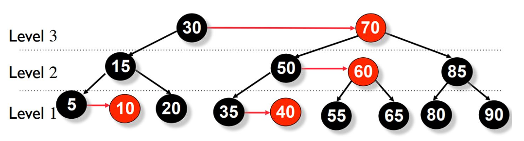
Building the Huffman Tree

Given the string "ADDAABBCCBAAABBCCCBBBCDAADDEEAA", the frequency table is:

Character	Frequency
A	10
B	8
C	6
D	5
E	2

The tree-building algorithm:

1. Create a leaf node for each character, weighted by frequency.
2. Extract the two nodes with the lowest weights $x$ and $y$.
3. Create a new internal node $z$ with weight $w(z) = w(x) + w(y)$; $x$ become the left child, $y$ the right child.
4. Insert $z$ back into the priority queue.
5. Repeat until only one node remains - this is the root.

The resulting Huffman Tree and bit-code table:

Character	Huffman Code	Length
A	11	2 bits
B	10	2 bits
C	00	2 bits
D	011	3 bits
E	010	3 bits

Compared to ASCII (8 bits/char), we now use an average of roughly 2.3 bits/char - a compression ratio exceeding 70%.

Theorem: Properties of the Huffman Tree

The Huffman tree produced by this greedy algorithm satisfies:

• It is a (every internal node has exactly 2 children).
• High-frequency nodes are positioned near the root (short paths → short codes).
• Low-frequency nodes are positioned far from the root (long paths → long codes).
• Total node count $= 2n - 1$ where $n$ is the number of distinct characters.

This tree is provably optimal - no other prefix-free code achieves a lower expected codeword length for the given frequency distribution.

Compression Algorithm

Step 1: Scan data → build frequency table
Step 2: Build Huffman Tree from frequency table
Step 3: Generate bit-code table by tree traversal
        (left edge = 0, right edge = 1)
Step 4: Re-scan data → replace each character with its bit code
Step 5: Store Huffman Tree metadata for decompression

Limitations of Classic Huffman

While optimal, classic huffman has real-world drawbacks:

• Two-pass requirement - must scan all data before encoding a single bit.
• Must store the tree - the decoder needs the frequency table or tree, adding overhead to the compressed file.
• Not streamable - the complete input must be available upfront.

This is where Adaptive Huffman comes in.

5. Adaptive Huffman - The Online Learner

Motivation

What if data arrives in a stream - live sensor readings, real-time network traffic, or keyboard input? Classic Huffman can’t handle this because it needs to see everything first. Adaptive Huffman (proposed by Faller in 1973, refined by Gallager in 1978, and perfected by Knuth in 1985 as the FGK algorithm; further optimized by Vitter in 1987) solves this beautifully.

Key Differences from Classic Huffman

Property	Classic Huffman	Adaptive Huffman
Passes over data	2 (frequency scan + encode)	1 (encode on-the-fly)
Tree stored in output?	Yes	No
Supports streaming?	No	Yes
Tree updates	Never	After every symbol

The NYT Node - The Secret Weapon

The Adaptive Huffman tree always contains a special leaf called the NYT (Not Yet Transmitted) node with weight 0. It acts as a placeholder for all characters not yet seen. When a new character is encountered for the first time, its code is transmitted as:

[NYT path bits] + [8-bits ASCII of the character]

After transmission, the NYT node splits into a new NYT node and a leaf node for the new character.

The Sibling Property - Maintaining Tree Validity

After every character is processed, the tree must maintain the sibling property: nodes are ordered by weight in increasing order form bottom-to-top and left-to-right. If a weight increment violates this order, the offending node is swapped with the farthest node of the same weight before incrementing.

Update procedure for node $p$ (after encoding character $c$):

loop while p ≠ NULL:
  1. If p is root: increment weight, stop
  2. Find the farthest node q (bottom-up, left-to-right) with the same weight as p (excluding p's parent)
  3. Swap p and q
  4. Increment p's weight
  5. Move p to its parent

Compression Flow

Step 1: Initialize tree with single NYT node
Step 2: For each character c in the input:
  2.1 Read c
  2.2 Encode c:
    - If c IS in tree: output its Huffman path code
    - If c is NOT in tree: output NYT path + ASCII(c)
  2.3 Update tree (split NYT if new, then propagate weights up)

Why This Is Clever

The decoder mirros exactly the same update steps as the encoder. Since both sides apply identical transformations to the same initial tree, they stay perfectly synchronized - no side-channel information needed.

6. Algorithm Comparison at a Glance

Research has shown that LZW achieves higher compression ratios than RLE and classic Huffman for text data when evaluated individually. But the best choice always depends on use cases:

Algorithm	Time Complexity	Space	Best For	Real-World Use
RLE	$O(n)$	$O(1)$	Repetitive data, images	BMP, PCX, fax
LZW	$O(n)$	$O(d)$ dict	Text, mixed data	GIF, TIFF, compress
Huffman	$O(n \log n)$	$O(k)$ tree	Text, entropy-near-optimal	ZIP, JPEG (part of), MP3
Adaptive Huffman	$O(n \log n)$	$O(k)$ tree	Streaming, real-time	Network protocols

Where $n$ = input length, $d$ = dictionary size, $k$ = alphabet size.

Where You’ve Already Seen These

LZW and its descendants form the basis of several ubiquitous compression schemes, including the one used in GIF and the DEFLATE algorithm used in PNG and ZIP.

Huffman coding is used in conventional compression formats like GZIP, BZIP2, PKZIP, JPEG, and MPEG-2.

GIF images are compressed using the lossless LZW data compression technique, while PNG is a lossless format the uses ZIP/DEFLATE compression, which is slightly more effective than LZW.

7. A Deeper Mathematical Perspective

Information Theory Foundation

All of these algorithms are chasing the same theoretical limit: Shannon’s entropy. For a source with symbols $s_1, s_2, \ldots, s_k$ and probabilities $p_1, p_2, \ldots, p_k$, the entropy is:

\[H = -\sum_{i=1}^{k} p_i \log_2 p_i \quad \text{(bits per symbol)}\]

Huffman coding is provably optimal in the sense that the expected codeword length $\bar{L}$ satisfies:

\[H \leq \bar{L} < H + 1\]

You can never do better than entropy (it’s a fundamental limit), and Huffman gets within 1 bit of it. Arithmetic coding can get even closer, but that’s a topic for another post!

Why RLE Can Make Files Lagger

Consider encoding "ABCDEF" with RLE: the ouput would be 1A1B1C1D1E1F - twice as long as the input! This is why RLE is only applied when there’s string evidence of repetition (e.g., in image formats where solid-color regions are common).

❮ ❯