Hash Table

In our journey through data structures, we have encountered various paradigms for storing and retrieving memory. Linear structures like standard Arrays provide contiguous memory layouts for lightning-fast indexing, but the degrade to a sluggish $O(n)$ linear scan when searching for a specific key. Linked Lists solve the problem of dynamic allocation but force the CPU into inefficient, $O(n)$ pointer-chasing.

Even as we leveled up to complex, self-balancing hierarchical structures like the B-Tree, we hit a mathematical ceiling. Their retrieval time is inherently bottlenecked at $O(\log n)$ because they strictly rely on key comparisions (evaluating whether to branch left or right). As datasets scale to millions of records, this traversal still incurs a heavy computational cost.

To shatter this logarithmic barrier and achieve a constant time complexity of $O(1)$ for key-based searching, we must abandon comparisons altogether. Instead, we use mathematics to map a Key directly to a physical Memory Address. The data structure that performs this magic is the Hash Table.

1. Modular Arithmetic

To build a Hash Table, we must rely on Discrete Mathematics, specifically Modular Arithmetic.

By definition, for a positive interger $n \in \mathbb{N}$, two intergers $a, b \in \mathbb{Z}$ are considered congruent modulo $n$ if they yield the same remainder when divided by $n$.

For example, $11 \equiv 8 \pmod 3$ because both 11 and 8 leave a remainder of 2 when divided by 3. This congruence property allows us to compress an infinite universe of keys into a finite array space using the modulo operator.

2. Hashing

A Hash Table is essentially a contiguous array of size $m$. The core engine driving this structure is the Hash Function ($h$).

The hash function acts a mapping mechanism from a universe of keys $U$ to a specific address: $h: U \to {0, 1, \dots, m-1}$.

An exceptional hash function must meet three criteria:

3. Load factor & The Co

2. Anatomy of a Hash Table & Hash Functions

A Hash Table is essentially a contiguous array of size $m$[cite: 81]. The core engine driving this structure is the Hash Function ($h$).

The hash function acts as a mapping mechanism from a universe of keys $U$ to a specific address: $h: U \to {0, 1, \dots, m-1}$[cite: 83]. [cite_start]An exceptional hash function must meet three criteria[cite: 156]:

1. [cite_start]Deterministic: The same input must always yield the exact same $h(k)$[cite: 160].
2. [cite_start]Uniform Distribution: It should distribute keys evenly across the addresses to minimize collisions[cite: 162].
3. [cite_start]Computationally Fast: The time cost to calculate $h(k)$ should ideally be $O(1)$[cite: 166].

Typecasting and Hashing Algorithms

[cite_start]Since hash functions perform mathematical operations, all keys (like strings) must be converted into unsigned integers[cite: 122].

• For Strings (Polynomial Hashing): Let $s$ be a string of length $m$ and $b$ be a constant base. The hash is calculated as: [cite_start]$f(s) = (s_0 \cdot b^{m-1} + s_1 \cdot b^{m-2} + \dots + s_{m-1}) \pmod{2^n}$[cite: 152, 153]. [cite_start]Performance Note: This is efficiently computed using Horner’s method to reduce multiplication operations[cite: 154].

• [cite_start]For Integers (Knuth’s Multiplicative Hash): Introduced by Donald Knuth, this method relies on a fractional constant $A$ (where $0 < A < 1$)[cite: 194]. [cite_start]$h(k) = \lfloor m \cdot (k \cdot A \pmod 1) \rfloor$[cite: 193]. [cite_start]The optimal value for $A$ is the golden ratio: $A = (\sqrt{5} - 1) / 2 \approx 0.618033$[cite: 195].

3. Load Factor & The Collision Problem

Two metrics govern the performance of a hash table:

• Load Factor ($\alpha$): Defined as the ratio of the number of elements $n$ to the table size $m$ ($\alpha = \frac{n}{m}$)[cite: 88].
• Collision: This occurs when two distinct keys $x \neq y$ generate the exact same hash code $h(x) = h(y)$[cite: 90].

Because the key universe $U$ is vastly larger than the table size $m$, collisions are mathematically inevitable. To resolve memory allocation conflicts during collisions, system engineers employ two primary architectural paradigms.

4. Collision Resolution I: Separate Chaining

[cite_start]The logic behind Separate Chaining is intuitive: if multiple keys map to the same address, we store them together by creating a Linked List at that specific index[cite: 208].

From a low-level C/C++ perspective (using Procedural Programming without heavy OOP classes), the hash table array does not hold the actual data. Instead, it holds pointers to the head of a linked list:

template <typename K, typename V>
struct HashNode {
    K key;
    V value;
    HashNode* next; // Pointer to the next collision node
};

// The Hash Table is an array of pointers #define M 1024 HashNode<K, V>* table[M];

2. Mathematical anatomy of a B-Tree

Properties of a B-Tree

A B-Tree of order $m$ is a highly constrained m-Way Search Tree. To guarantee structural balance ($O(\log m)$ time complexity), it must satisfy strict mathematical invariants:

1. Root Constraint: The root must have at least 2 children (unless it is a leaf).
2. Node Capacity Limits:
   • Every node has at most $m$ children and $m-1$ keys.
   • Every internal node (except the root) must be at least half-full. It must have at least $\lceil m/2 \rceil$ children and $\lceil m/2 \rceil - 1$ keys.
3. Perfect Leaf Alignment: All leaf nodes must exist strictly at the exact same level. This property is what defines it as “perfectly balanced”.

Following is an example of a B-Tree of order 4:

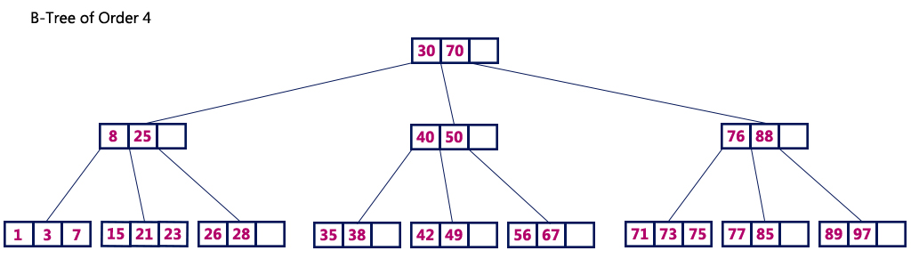
We can see in the above diagram that all the leaf nodes are at the same level and all non-leaf nodes have no empty sub-tree and have number of keys one less than the number of their children.

B-Tree’s Height theorems

The absolute guarantee of a B-Tree’s performance lies in its height bounds. Let $n$ be the total number of keys in a B-Tree of order $m$ and height $h$ (assuming the root is at level 1). Let the minimum degree be $t = \lceil m/2 \rceil$.

1. Minimum Height: The tree is as flat as possible when every node is completely saturated with $m - 1$ keys. The height is bounded by:

\[h \ge \log_m(n+1)\]

1. Maximum Height: The tree is as tall as possible when every internal node contains the bare minimum of keys ($t - 1$). By summing the nodes at each level, mathematicians have proven the upper bound:

\[h \le \log_t \left( \frac{n+1}{2} \right) + 1\]

These theorems mathematically prove that the height grows logarithmically.

Complexity analysis

Define a B-Tree

From a C++ low-level perspective, we must modify our previous mWayNode by introducing a boolean flag to identify leaf status, which dictates our traversal and splitiing logic:

#define M 4
struct BTreeNode {
  int count;               // Current number of keys
  int keys[M - 1];         // Array of sorted keys 
  BTreeNode* children[M];  // Array of pointers to subtrees  
  bool isleaf;             // True if node is a leaf
};

3. Operation in B-Tree

Searching

Searching in a B-Tree is a two-tier process that beautifully balances fast CPU operations with slow Disk I/O.

When looking for a target key $X$, starting from the root:

1. In-Memory Binary Search: Once a node (a disk page) is loaded into RAM, we perform a standard Binary Search within its sorted keys array. Because this happens entirely in the CPU cache, it is blindingly fast.
2. Evaluation:
   • If $X$ matches a key, the search terminates successfully.
   • If $X$ is not found, the binary search gives us the correct routing index $i$ where $k_{i-1} < X < k_i$.
3. Disk Traversal: We look at the pointer $P_i$. If the current node’s isleaf flag is true, the pointer is nullptr and the key does not exist. Otherwise, we command the hardware to fetch the child node $P_i$ from the disk into RAM, and recursively repeat the process.

Insertion

Unlike a Binary Search Tree that growns downwards, a B-Tree growns upwards.

When inserting a new key $X$:

1. Traverse down to the appropriate leaf node.
2. If the leaf is not full, insert $X$ into the array.
3. The Split: If the leaf is full (an overflow condition), we temporarily insert $X$ to find the median key. The node is violently split into two halves.
4. Promotion: The median key is stricly pushed up to the parent node. If the parent is also full, the split cascades upwards. If the root splits, a new root is created, increasing the height by 1.

Deletion

Deletion might cause a node to fall below its minimum threshold. This triggers an underflow state.

The rescue operation has two phase:

1. Borrowing: The deficient node looks to its immediate sibling. If a sibling has spare keys, we perform a rotation: pull a key from the sibling up to the parent, and pull the parent’s separating key down.
2. Merging: If both siblings are at minimum capacity, we merge the deficient node, its sibling, and the separating key from the parent into a single node. This removes a key from parent, potentially causing the parent to underflow, cascading the deletion upwards.

❮ ❯